Building Distributed Measurement Systems
Overview
Contents
- Centralized Versus Distributed Measurement Systems
- Requirements for Building Distributed Systems
- NI Products for Distributed Measurement Systems
- Related Information
Centralized Versus Distributed Measurement Systems
A basic measurement system consists of several necessary components that ensure operators get reliable, quality information from their tests. Starting with the unit under test (UUT), there are sensors that are wired to signal conditioning (sensor excitation, filtering, and so on required for quality sensor measurements). The signal conditioning sends these cleaned up signals to a data acquisition system, which turns the analog sensor signals into a digital signal that the computer can analyze or save for later. Additionally, operators use a user interface component to interact with the data acquisition system.
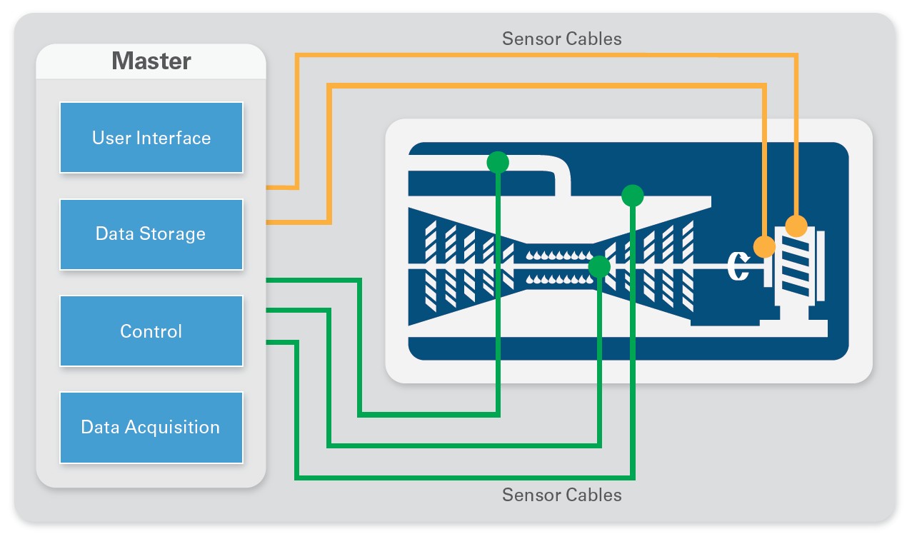
Figure 1. A centralized measurement system brings all the components together into a single system, usually some distance away from the unit under test.
Traditional data acquisition systems use a centralized architecture with large racks of measurement hardware and computers in a central control room. The advantages of these systems are that they are generally removed from the rigors of the testing environment and are easier to maintain. However, these centralized systems also can introduce excessive cost and complexity to your measurement systems.
Distributed systems place the data acquisition hardware around the UUT, often in the test environment and as close to the measurement sensor as possible. They interact with the UUT locally and receive commands from or send messages or data for logging back to a central server where the test operator is located. This architecture can offer several advantages over a centralized system. By breaking the large centralized system into distributed smaller systems, you create smaller, cheaper subsystems that you can more easily replace and maintain should one fail. You also reduce wiring cost by running a single communication cable to the distributed subsystems rather than laying possibly hundreds of sensor wires throughout your test cell. This reduction in cabling can lower costs and, more importantly, increase measurement accuracy because the shorter sensor wires to the distributed systems are less prone to noise, interference, and signal loss. Finally, a distributed system can help offload processing from a main central computer. Many distributed data acquisition systems also have onboard intelligence that can be used to run analysis or reduce data to just key values before uploading it to the central system. This allows your central computer to be substantially cheaper and faster than if it had to process raw measured channels as they came in while also handling user interface and data storage.
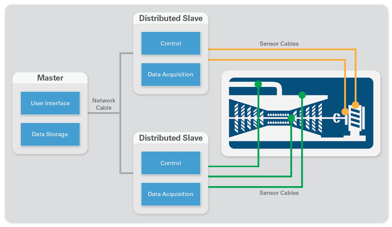
Figure 2. A distributed architecture separates the system components and places the measurement devices near the physical measurement being made.
Requirements for Building Distributed Systems
When selecting data acquisition hardware for a distributed measurement system, you must keep in mind specific requirements. Whereas localized signal conditioning and data acquisition are required by the very nature of the system, other features like the ability to synchronize measurements across all of the distributed nodes, ruggedness, and onboard processing can be selected and customized to meet your application needs. The network chosen to distribute and communicate with your nodes can also be an important decision, depending on the application and its requirements.
Localized Signal Conditioning and Data Acquisition
In a distributed measurement system, the sensor signal conditioning and data acquisition are located within nodes close to the sensors making the measurements. Signal conditioning can be positioned either external to the data acquisition devices, or can be internal to them. By integrating signal conditioning into the data acquisition devices, you can reduce system complexity and cost. Purchasing integrated signal conditioning means that the vendor has done the integration, testing, and certification for you, making it much easier to design and deploy your test system. Often, the total system cost is also reduced by purchasing components with integrated signal conditioning because of the economics scale vendors have over end users.
Ruggedness
Distributed systems tend to be located within the same test environments as the UUTs, so as to get as close to the sensors as possible. This often means that the data acquisition equipment can be exposed to harsh and demanding conditions where standard desktop equipment would give inaccurate data or fail entirely. Ensuring that your signal conditioning and data acquisition equipment can survive your test environment can help ensure you get accurate data the first time and eliminate the need for costly retests. Possible requirements for your system could include extreme temperature ranges for product validation testing, shock and vibration survivability if the system is to be mounted directly to a machine, or hazardous location certifications to ensure the system can safely operate in marine or explosive environments.
Although it is possible to design enclosures for any data acquisition system to meet these ruggedness requirements, it is often cheaper to purchase a system already tested and certified to survive the conditions. In developing and integrating your own ruggedness solutions, design, materials, testing, and compliance costs can quickly add up, in addition to the time to properly go through these steps. Vendors can amortize these costs over thousands of units, meaning they can offer the same benefits at a lower price.
Learn more about ruggedness and how to choose the right system for your environment.
Synchronization
Synchronization, at its most basic level, is ensuring that all pieces of a system have the same concept of time, usually by sharing clocks and trigger signals. It is often required in large measurement systems so that data taken throughout the test can be properly correlated and analyzed. Without proper synchronization, there is no way to know if two measurements happened simultaneously or, in the case of stimulus/response type testing, which stimulus the measurement is a response of. For example, Boeing used a large array of distributed microphone systems to triangulate the major noise sources of airplanes in flyover testing by measuring the delay for the sound of the plane to reach the different microphones. If the distributed microphone nodes were not properly synchronized, there would be no way to properly measure the delay between different nodes because they would not have the same concept of time.
With centralized measurement systems, synchronization is fairly straightforward because most systems are in the same chassis. A distributed system has inherent difficulties that must be overcome to synchronize systems over sometimes long distances. You can choose from several types of synchronization for use in distributed systems including software, time-based, and signal-based.
Software synchronization relies on data acquisition software to send a start trigger to all devices at the same time. This is the poorest implementation of synchronization and is generally on the order of milliseconds. Because no information is shared between distributed subsystems, their internal clocks can drift over time, reducing your synchronization over the course of the measurement.
Time-based synchronization gives system components a common reference for time from a known clock source. You can then generate events, triggers, and clocks based on this common reference time. For long distances, you can use a variety of time references including GPS, IEEE 1588v2, IEEE 802.1AS, and IRIG-B to correlate and synchronize measurements anywhere in the world with absolute timing with or without a direct connection between the measurement systems. Time-based synchronization is most often used to reduce or eliminate the need to run synchronization cabling between subsystems, instead using network cables already in place or wireless synchronization clocks such as GPS.
Signal-based synchronization physically connects clocks and triggers between subsystems. Typically, this provides the highest precision synchronization, but requires signal wire connecting your subsystems to share the synchronization signals. The downside of signal-based synchronization is there may be skew and uncertainly from routing delays along the physical signal wire.
Learn more about the different types of synchronization.
Onboard Intelligence
Though not required to build a distributed system, data acquisition nodes with onboard intelligence can have significant benefits for your system. By placing intelligence on your nodes, you give them the ability to distribute data analysis and possibly control your subsystems, offloading it from the central computer. Distributed data analysis can reduce the amount of data you are sending back to the main computer over the network, significantly reducing the network traffic and required bandwidth. Rather than pass all the raw measured waveforms across the network, you can perform analysis locally and then pass back only results to the central computer for storage or integration into larger analysis and decision making. Of course, you can also always send raw waveforms over the network should the situation arise.
You can choose from three different levels of onboard intelligence, each offering different levels of flexibility and complexity.
Windows is likely the most familiar system choice. With Microsoft continuing to invest in its Windows embedded system, there are limited reliability concerns with using it for a measurement application. Additionally the ability to run a user interface directly on it could be a benefit for your application, as well as being able to run common .exe windows applications without having to worry about coding for other more common embedded systems.
Real-time OSs (RTOSs) are more likely to be used in distributed measurement systems because of their reliability and deterministic nature. By guaranteeing that commands and measurements are executed within certain time constraints, real-time systems are well suited to a measurement system with a high need for uptime and reliability or with deterministic tight timing requirements.
FPGAs are reprogrammable silicon chips and offer the ultimate in flexibility and customizability for distributed systems. Reprogrammable silicon also has the same flexibility of software running on a processor-based system, but it is not limited by the number of processing cores available. Unlike processors, FPGAs are truly parallel in nature, so different processing operations do not have to compete for the same resources. Additionally, because the code is written into silicon chips, an FPGA can measure, analyze, and then output data much faster than a processor-based system.
Network
The network you distribute your system with is just as critical as the hardware that is distributed. Depending on the distribution distance, data bandwidth, synchronization, and determinism requirements, there are a wide variety of networks that you could choose. Though there are communication networks based on serial communication technologies, this article focuses on Ethernet-based technologies that continue to become more and more commonplace and can offer more benefits than serial communication and at a lower price.
Ethernet (UDP) is standard Ethernet technology that serves to only broadcast data. UDP is a multicast protocol that routes packets from the controller to multiple destinations. This is an efficient communication method for one controller to broadcast data to multiple receivers, but it can create broadcast storms that consume network bandwidth. There is no guarantee that information has been received and so should be used only for slowly updating noncritical data.
Ethernet (TCP/IP) is also standard Ethernet technology that is better suited for critical data. TCP/IP buffers data and implements a handshake process between senders and receivers to ensure data is properly received and can work well for crucial data and be used for either single-point or streaming data.
OPC (OLE for Process Control) is a standard that was developed to allow different devices from different vendors to communicate with each other over a common vendor agnostics protocol. Most suppliers of industrial data acquisition and control devices are designed to work with OPC.
Modbus is a nondeterministic protocol with a simple client/server architecture that uses standard Ethernet hardware and the TCP/IP transport layer. It is ideal for applications that need to mix hardware from multiple vendors and require low to moderate bandwidth.
EtherCAT was developed by Beckhoff and integrates synchronization and deterministic data transfer into a master/slave architecture. EtherCAT is optimized for single-point communication and is common in applications with motion such as machine control.
NI Products for Distributed Measurement Systems
National Instruments has a wide variety of platforms and products that can be used to build high-quality distributed measurement systems. From the performance and high channel counts of PXI to the integrated signal conditioning and small form factor of NI CompactDAQ to the flexibility and customizability of CompactRIO, there is an NI platform that will work to help you meet your application needs.
NI PXI
NI PXI is a rugged PC-based platform built around the PXI and PXI Express open standards. A single system consists of a chassis, controller, and up to 18 high-performance, high-channel-count data acquisition cards. Additionally, you can network and tightly synchronize chassis together to form even larger channel count distributed subsystems if required. PXI controllers offer a wide variety of both Windows and RTOS onboard processing performance from single-core 1.66 GHz atom processors to quad-core 2.3 GHz processors. To meet your test and distributed measurement needs, you can choose from over 450 NI PXI modules, including those with integrated signal conditioning for your sensors.
NI PXI systems give you the best measurement, synchronization, and processing performance for developing distributed measurement systems while supporting all of the major industrial network standards.
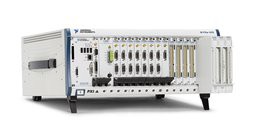
Figure 3. NI PXI gives you the highest performance and channel count available for distributed measurement nodes.
NI CompactDAQ
NI CompactDAQ is a modular data acquisition system that consists of a chassis, NI C Series data acquisition modules, and an optional real-time or Windows controller. Designed with a smaller footprint and more rugged specifications than PXI, NI CompactDAQ is designed to allow you to take reliable measurements anywhere from the lab bench to the rugged test cell. With over 60 C Series I/O modules available for measuring anything from standard voltage to strain, temperature, and vibration, you can build a custom distributed measurement solution that meets your application needs with integrated signal conditioning.
NI CompactDAQ can operate either tethered to a host computer via USB, Ethernet, or WiFi or operate as a stand-alone system with a Windows or RTOS for onboard processing, data reduction, and industrial network communication.
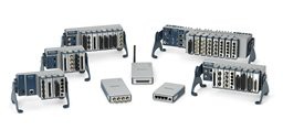
Figure 4. NI CompactDAQ is a rugged, distributable form factor that can be customized to connect to any type of physical measurement.
NI CompactRIO
NI CompactRIO systems consist of an embedded controller for communication and processing, a reconfigurable chassis housing the user-programmable FPGA, and the same hot-swappable C Series I/O modules used on the NI CompactDAQ platform. With a wide variety of controller options from value-based to high-performance dual-core Windows or real-time systems, you can be assured that CompactRIO can handle any onboard processing or industrial networking your application requires. You can use the onboard FPGA to further add custom signal processing, timing constraints, or protocols for the ultimate in flexibility.
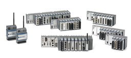
Figure 5. NI CompactRIO offers the ultimate in flexibility and onboard processing in a rugged, distributable form factor.
Related Information
Selecting rugged measurements hardware for your distributed system
Synchronizing distributed subsystems
Learn more about NI platforms:
View NI PXI chassis options for prices and specifications.
View NI CompactDAQ chassis options for prices and specifications.
View NI CompactRIO chassis options for prices and specifications.