Using Fast Fourier Transforms and Power Spectra in LabVIEW

LabVIEW and its analysis VI library provide a complete set of tools to perform Fourier and spectral analysis. The Fast Fourier Transform (FFT) and Power Spectrum VIs are optimized and their outputs adhere to the standard DSP format.

FFT is a powerful signal analysis tool, applicable to a wide variety of fields including spectral analysis, digital filtering, applied mechanics, acoustics, medical imaging, modal analysis, numerical analysis, seismography, instrumentation, and communications.

The LabVIEW analysis VIs, located on the Functions»Signal Processing palette, maximize analysis throughput in FFT-related applications. This document discusses FFT properties, how to interpret and display FFT results, and how to manipulate FFT and power spectrum results to extract useful frequency information.

FFT Properties

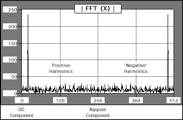
The fast Fourier transform maps time-domain functions into frequency-domain representations. FFT is derived from the Fourier transform equation, which is:
where x(t) is the time domain signal, X(f) is the FFT, and ft is the frequency to analyze.

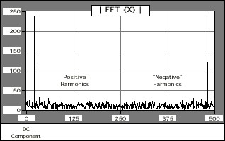
Similarly, the discrete Fourier transform (DFT) maps discrete-time sequences into discrete-frequency representations. DFT is given by the following equation:

where x is the input sequence, X is the DFT, and n is the number of samples in both the discrete-time and the discrete-frequency domains.

Direct implementation of the DFT, as shown in equation 2, requires approximately n² complex operations. However, computationally efficient algorithms can require as little as n log2(n) operations. These algorithms are FFTs, as shown in Equations 4,5, and 6.

Using the DFT, the Fourier transform of any sequence x, whether it is real or complex, always results in a complex output sequence X of the following form:

An inherent DFT property is the following:

where the (n-i)th element of X contains the result of the -ith harmonic. Furthermore, if x is real, the ith harmonic and the -ith harmonic are complex conjugates:


Consequently,

and

These symmetrical Fourier properties of real sequences are referred to as conjugate symmetric (equation 5), symmetric or even-symmetric (equation 6), and asymmetric or odd-symmetric (equation 7).

FFT Output Format

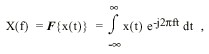
The output format of the FFT VI can now be described with the aid of equation 4. If the total number of samples, n, of the input sequence, x, is even, the format of the complex output sequence, X, and the interpretation of the results are shown in Table 1.


Figure 1 represents the output format described in Table 1 for n = 512.



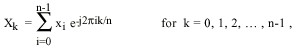
If the total number of samples, n, of the input sequence, x, is odd, the format of the complex output sequence, X, and the interpretation of the results are shown in Table 2.


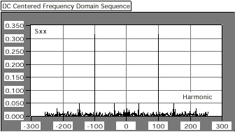
Figure 2 represents the output format described in Table 2 for n = 500.
In most applications, you perform FFT and spectral analysis only on real-valued, discrete-time sequences. This section describes the following three common formats for displaying the FFT results of real-valued input sequences: standard, double-sided, and single-sided.

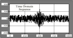
The time-domain signal shown in Figure 3 demonstrates the three methods by which FFT results can be displayed graphically. The time-domain signal has a signal of interest buried in the noise that is easily identified in the frequency domain. Based on frequency information, digital filtering can remove the noise from the signal.


Standard Output
Standard output is the format for even and odd-sized discrete-time sequences, described in Tables 1 and 2 of this document. This format is convenient because it does not require any further data manipulation.

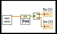
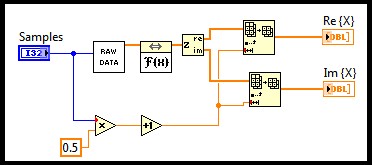
To graphically display the results of the FFT, wire the output arrays to the waveform graph, as shown in Figure 4. The FFT output is complex and requires two graphs to display all the information.


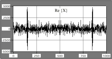
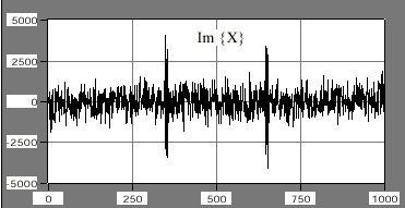
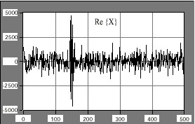
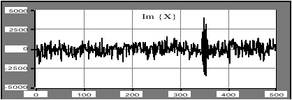
Figures 5 and 6 are plots of the real and imaginary portions, respectively, of the FFT VI results. The symmetrical properties summarized in equations 5 through 7 are clearly visible in the plots.



Double-Sided Output
The FFT integral, shown in equation 1, has a frequency range of . Presenting FFT results in this frequency range is a double-sided format, as shown in Figure 7.


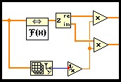
You can obtain double-sided output format from the standard output by recalling the identity X_-i = X_n-i. To present the data in a double-sided format, you must split the arrays at their center point into two portions, corresponding to the positive and negative frequencies, and reverse the array order by appending the positive frequencies to the negative frequencies. You can do this in LabVIEW with the Split 1D Array and Build Array functions, as shown in Figure 8.


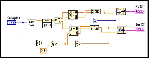
The lower portion of the block diagram finds the index at which the arrays need to be split. This technique works for both an even and odd number of samples.

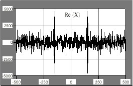
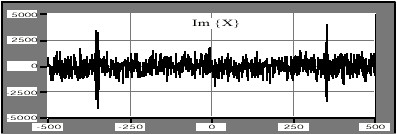
The results of processing the data using the block diagram shown in Figure 8 are shown in figures 9 and 10, corresponding to the real and imaginary parts, respectively. Both graphs display the frequency information from - (n ÷ 2) to (n ÷ 2) and the symmetry properties about zero are clear.


Single-Sided Output
Almost half the information is redundant in standard and double-sided output formats. This is clear from equations 5, 6, and 7. The data is conjugate symmetric about the (n÷2)^th harmonic, also known as the Nyquist harmonic. Therefore, you can discard all the information above the Nyquist harmonic because you can reconstruct it from the frequencies below the Nyquist harmonic. Displaying only the positive frequencies gives you single-sided output.

The block diagram shown in Figure 11 uses the Array Subset function to select all the elements corresponding to the positive frequencies, including the DC component. Like the double-sided case, the lower portion of the block diagram selects the total number of elements in the subset and works for both an even and odd number of samples.


The results of processing the data using the block diagram in Figure 11 are shown in Figures 12 and 13, corresponding to the real and imaginary parts, respectively. Both graphs display the frequency information from 0 to (n ÷ 2), which is approximately half the points presented in standard and double-sided outputs.


Note: You must pay careful attention if you make measurements with single-sided data because the total energy at a particular frequency is equally divided between the positive and negative frequency, DC and Nyquist components excluded.

Fourier Analysis Using FFTs

To analyze a discrete-time signal using FFT, equation 2 must include a 1/n scaling factor, where n is the number of samples in the sequence. Figure 14 shows a block diagram segment that scales the FFT results by the 1/n factor. You can apply the same scaling factor to the double-sided and single-sided formats.


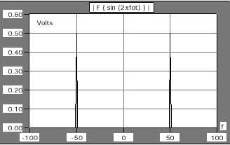
For example, the FFT of the sine wave shown in Figure 15 is the following equation:

where
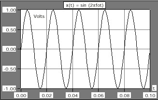
Figure 16 shows the double-sided Fourier analysis of the sinusoidal waveform.In many applications it is not convenient to think in terms of complex data. Instead, you can present complex data as magnitude and phase data. To illustrate this point, Figures 17 and 18 show the frequency response of a filter in terms of complex data. Figures 19 and 20 show the same frequency response as magnitude and phase data.

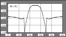
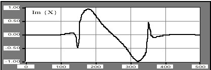
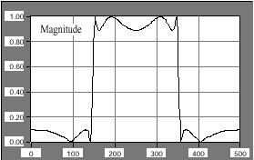
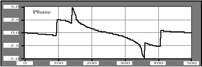
Although the phase information may not appear to carry useful information, the filter's magnitude-frequency response is clearly that of a bandpass filter.

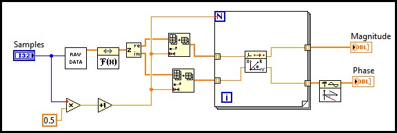
You obtain magnitude and phase information from complex data using the 1D Rectangular To Polar VI. Because phase information is computed using an arc tangent function, and the arc tangent function results are in the -p to p range, you can use the Unwrap Phase VI to smooth out some of the discontinuities that might arise when converting complex data to magnitude and phase data.

Figure 21 shows how to use the 1D Rectangular To Polar and the Unwrap Phase VIs to convert complex data into magnitude and phase format. Figure 21 shows the single-sided output format, but you also can apply the same technique to the standard output and double-sided output formats.


Power Spectrum
Use the Power Spectrum VI, which is closely related to the FFT, to calculate the harmonic power in a signal. The power spectrum, Sxx(f), of a time domain signal, x(t), is defined using the following equation:

where
Because the power spectrum format is identical to the real part of the FFT, the description of standard, double-sided, and single-sided formats applies to the Power Spectrum VI. Furthermore, the single-sided format uses less memory because this format eliminates redundancy while retaining the complete power spectrum information.

The Power Spectrum VI calculates the harmonic power in discrete-time, real-valued sequences. Figure 22 shows the single-sided output of the power spectrum of two 1-V peak sinusoids -- one with 150 cycles and one with 250 cycles. The total power for each one of these sinusoids is 2 ´ 0.25 W.


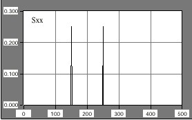
The discrete implementation of the power spectrum, Sxx, is given by the following equation:


where x is the discrete-time, real-valued sequence and n is the number of elements in x.

Unlike the FFT, power spectrum results are always real. The Power Spectrum VI runs faster than the FFT VI because it performs the computation in place and does not need to allocate memory to accommodate complex results. However, you cannot reconstruct phase information output sequence of the power spectrum. Use the FFT if phase information is important.

Converting Magnitude Information to Decibels

Use 10 * log[10] X[i] and 20 * log[10] X[i] to convert 1D numeric arrays into decibels (dB), which is a common unit for representing power ratios. Log[10] can be computed using the Logarithm Base 10 function, located on the Functions»Numeric»Logarithmic palette.

Use 10 * log[10] X[i] to convert magnitude squared or power values, such as acoustic pressure waves, to decibels. Use 20 * log[10] X[i] to convert magnitude or amplitude values, such as voltages or currents, to decibels.

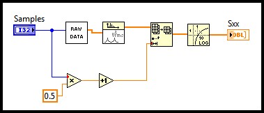
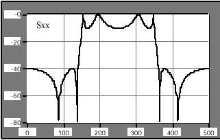
The block diagram in Figure 23 shows an example that converts the result of the power spectrum to decibel notation. Figure 24 shows the results. In Figure 23, the Raw Data icon represents your array, X[i], and the 10LogX VI can be built using the Logarithm Base 10 function.

The discrete implementation of the FFT maps a digital signal into its Fourier series coefficients or harmonics. The arrays involved in FFT-related operations do not contain discrete-time or discrete-frequency information. You can use modern acquisition systems, whether they use add-on boards or instruments to capture the data, to control or specify the sampling interval, Dt, and obtain frequency scaling information from Dt.

Because an acquired array of samples commonly represents real-valued signals acquired at equally spaced time intervals, you can determine the value corresponding to the observed frequency in Hertz. To associate a frequency axis to operations that map time signals into frequency domain representations, such as the FFT, power spectrum, and Hartley transforms, the sampling frequency, fs, must first be determined from Dt using the following equation:



The frequency interval is given by the following equation:

where n is the number of samples in the sequence.

Given the sampling interval, 1.000E-3, the block diagram shown in Figure 25 demonstrates how to display a graph with the correct frequency scale.


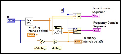
Thus, for the signal, x(t), represented in Figure 26, Figure 27 shows the resulting single-sided power spectrum graph with the correct frequency axis. The resulting frequency interval is 1.953E0.



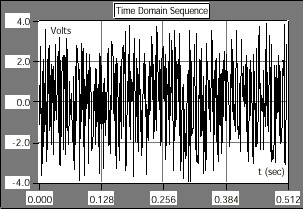
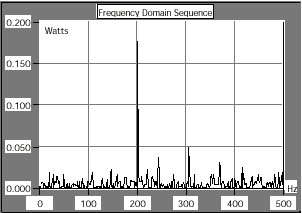
The sampling interval is the smallest frequency that the system can resolve through FFT or related routines. A simple way to increase the resolution is to increase the number of samples or increase the sampling interval.

Reader Comments | Submit a comment »

Awesome tutorial!
Who wrote this? Cyril? ANyway. It is VERY helpful! Nice job. See the sample here: http://zone.ni.com/devzone/explprog.nsf/6c163603265406328625682a006ed37d/433c2cb c5a1c4a49862569500035f715?OpenDocument Whoever wrote that is an absolute WIZARD. I just want to know how to replace the IIR with a REAL device. In short. Replace the IIR with a means to drive a system with a swept sin wave (just like input of IIR) and then measure the response with an Analog Input. Then this goes into the rest of the VI. Thanks, Dave korpi@starband.net
- Dave Korpi, Sierra Instruments. korpi@starband.net - Sep 10, 2002