Using the LabVIEW Shared Variable
Overview
LabVIEW provides access to a wide variety of technologies for creating distributed applications. The shared variable simplifies the programming necessary for such applications. This article provides an introduction to the shared variable and includes a discussion of its features and performance.
Using the shared variable, you can share data between loops on a single diagram or between VIs across the network. In contrast to many other data-sharing methods in LabVIEW, such as UDP/TCP, LabVIEW queues, and Real-Time FIFOs, you typically configure the shared variable at edit time using property dialogs, and you do not need to include configuration code in your application.
You can create two types of shared variables: single-process and network-published. This paper discusses the single-process and the network-published shared variables in detail.
Contents
- Creating Shared Variables
- Single-Process Shared Variable
- Network-Published Shared Variable
- The Shared Variable Engine
- Performance
- Benchmarks
Creating Shared Variables
To create a shared variable, you must have a LabVIEW project open. From the project explorer, right-click a target, a project library, or a folder within a project library and select New»Variable from the shortcut menu to display the Shared Variable Properties dialog box. Select among the shared variable configuration options and click the OK button.
If you right-click a target or a folder that is not inside a project library and select New»Variable from the shortcut menu to create a shared variable, LabVIEW creates a new project library and places the shared variable inside. Refer to the Shared Variable Lifetime section for more information about variables and libraries.
Figure 1 shows the Shared Variable Properties dialog box for a single-process shared variable. The LabVIEW Real-Time Module and the LabVIEW Datalogging and Supervisory Control (DSC) Module provide additional features and configurable properties to shared variables. Although in this example both the LabVIEW Real-Time Module and the LabVIEW DSC Module are installed, you can use the features the LabVIEW DSC Module adds only for network-published shared variables.
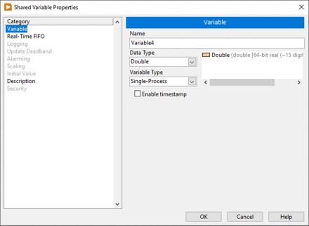
Figure 1. Single-Process Shared Variable Properties
Data Type
You can select from a large number of standard data types for a new shared variable. In addition to these standard data types, you can specify a custom data type by selecting Custom from the Data Type pull-down list and navigating to a custom control. However, some features such as scaling and real-time FIFOs will not work with some custom datatypes. Also, if you have the LabVIEW DSC Module installed, alarming is limited to bad status notifications when using custom datatypes.
After you configure the shared variable properties and click the OK button, the shared variable appears in your Project Explorer window under the library or target you selected, as shown in Figure 2.
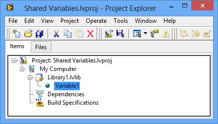
Figure 2. Shared Variable in the Project
The target to which the shared variable belongs is the target from which LabVIEW deploys and hosts the shared variable. Refer to the Deployment and Hosting section for more information about deploying and hosting shared variables.
Variable References
After you add a shared variable to a LabVIEW project, you can drag the shared variable to the block diagram of a VI to read or write the shared variable, as shown in Figure 3. The read and write nodes on the diagram are called Shared Variable nodes.
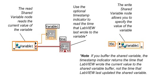
Figure 3. Reading and Writing to a Shared Variable Using a Shared Variable Node
You can set a Shared Variable node as absolute or target-relative depending on how you want the node to connect to the variable. An absolute Shared Variable node connects to the shared variable on the target on which you created the variable. A target-relative Shared Variable node connects to the shared variable on the target on which you run the VI that contains the node.
If you move a VI that contains a target-relative Shared Variable node to a new target, you also must move the shared variable to the new target. Use target-relative Shared Variable nodes when you expect to move VIs and variables to other targets.
Shared Variable nodes are absolute by default. Right-click a node and select Reference Mode»Target Relative or Reference Mode»Absolute to change how the Shared Variable node connects to the shared variable.
You can right-click a shared variable in the Project Explorer window and edit the shared variable properties at any time. The LabVIEW project propagates the new settings to all shared variable references in memory. When you save the variable library, these changes are also applied to the variable definition stored on disk.
Single-Process Shared Variable
Use single-process variables to transfer data between two different locations on the same VI that cannot be connected by wires, such as parallel loops on the same VI, or two different VIs within the same application instance. The underlying implementation of the single-process shared variable is similar to that of the LabVIEW global variable. The main advantage of single-process shared variables over traditional global variables is the ability to convert a single-process shared variable into a network-published shared variable that any node on a network can access.
Single-Process Shared Variables and LabVIEW Real-Time
In order to maintain determinism, a real-time application requires the use of a nonblocking, deterministic mechanism to transfer data from deterministic sections of the code, such as higher-priority timed loops and time-critical priority VIs, to nondeterministic sections of the code. When you install the LabVIEW Real-Time Module, you can configure a shared variable to use real-time FIFOs by enabling the real-time FIFO feature from the Shared Variable Properties dialog box. NI recommends using real-time FIFOs to transfer data between a time-critical and a lower-priority loop. You can avoid using the low-level real-time FIFO VIs by enabling the real-time FIFO on a single-process shared variable.
LabVIEW creates a real-time FIFO when the VI is reserved for execution (when the top-level VI in the application starts running in most cases), so no special consideration of the first execution of the Shared Variable node is needed.
Note: In legacy versions of LabVIEW (versions prior to 8.6), LabVIEW creates a real-time FIFO the first time a Shared Variable node attempts to write to or read from a shared variable. This behavior results in a slightly longer execution time for the first use of each shared variable compared with subsequent uses. If an application requires extremely precise timing, include either initial ”warm-up” iterations in the time-critical loop to account for this fluctuation in access times or read the variable at least once outside the time-critical loop.
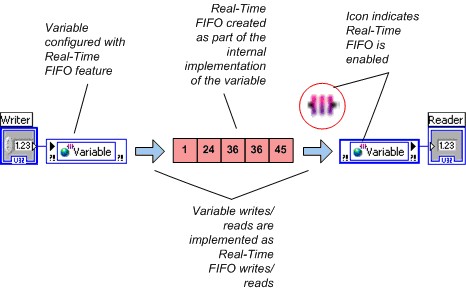
Figure 4. Real-Time FIFO-Enabled Shared Variables
LabVIEW creates a single, real-time FIFO for each single-process shared variable even if the shared variable has multiple writers or readers. To ensure data integrity, multiple writers block each other as do multiple readers. However, a reader does not block a writer, and a writer does not block a reader. NI recommends avoiding multiple writers or multiple readers of single-process shared variables used in time-critical loops.
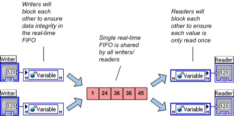
Figure 5. Multiple Writers and Readers Sharing a Single FIFO
By enabling the real-time FIFO, you can select between two slightly different types of FIFO-enabled variables: the single-element and the multielement buffer. One distinction between these two types of buffers is that the single-element FIFO does not report warnings on overflow or underflow conditions. A second distinction is the value that LabVIEW returns when multiple readers read an empty buffer. Multiple readers of the single-element FIFO receive the same value, and the single-element FIFO returns the same value until a writer writes to that variable again. Multiple readers of an empty multielement FIFO each get the last value that they read from the buffer or the default value for the data type of the variable if they have not read from the variable before. This behavior is shown below.
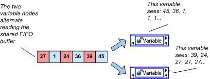
Figure 6. Last Read Behavior and the Multielement Real-Time FIFO Shared Variable
If an application requires that each reader get every data point written to a multielement FIFO shared variable, use a separate shared variable for each reader.
Network-Published Shared Variable
Using the network-published shared variable, you can write to and read from shared variables across an Ethernet network. The networking implementation is handled entirely by the network-published variable.
In addition to making your data available over the network, the network-published shared variable adds many features not available with the single-process shared variable. To provide this additional functionality, the internal implementation of the network-published shared variable is considerably more complex than that of the single-process shared variable. The next few sections discuss aspects of this implementation and offer recommendations for obtaining the best performance from the network-published shared variable.
NI-PSP
The NI Publish and Subscribe Protocol (NI-PSP) is a networking protocol optimized to be the transport for Network Shared Variables. The lowest level protocol underneath NI-PSP is TCP/IP and it has been thouroughly tuned with an eye toward performance on both desktop systems and NI's RT targets (see below for comparative benchmarks).
Theory of Operation of LogosXT
Figure 7 illustrates the software stack of the network shared variable. It is important to understand this because the theory of operation in play here is particular to the level of the stack called LogosXT. LogosXT is the layer of the stack responsible for optimizing throughput for the shared variable.
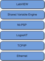
Figure 7. The Shared Variable Network Stack
Figure 8 shows the principle components of the LogosXT transmission algorithm. In essence, it is very simple. There are two important actors
- An 8 Kilobyte (KB) transmit buffer
- A 10 millisecond (ms) timer thread
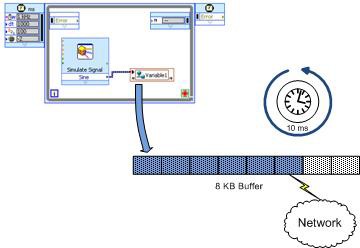
Figure 8. LogosXT Actors. The buffer will be transmitted if full or after 10ms has expired
These numbers were arrived at by thoroughly profiling various packet sizes and times to optimize for data throughput. The algorithm is as follows:
- IF the transmit buffer is filled to capacity (8KB) before the 10ms timer fires, then the data in that buffer is sent immediately to TCP on the same thread that initiated the write. In the case of the shared variable, the thread will be the shared variable engine thread.
- IF 10ms passes without the buffer ever filling up to capacity, then the data will be sent on the timer's thread.
Important note: There is one transmit buffer for all the connections between two distinct endpoints. That is, all the variables representing connections between two different machines will share one buffer. Do not confuse this transmit buffer with the Buffering property of shared variables. This transmit buffer is a very low level buffer that multiplexes variables into one TCP connection and optimizes network throughput.
It is important to understand the functionality of this layer of the network stack because it has side effects on the code on your LabVIEW diagram. The algorithm waits 10ms because it is always more efficient for throughput to send as much as possible in a single send operation. Every network operation has a fixed overhead both in time and in packet size. If we send many small packets (call it N packets) containing a total of B bytes, then we pay the network overhead N times. If instead, we send one large packet containing B bytes, then we only pay the fixed overhead once and overall throughput is much greater.
This algorithm works very well if what you want to do is stream data from or to a target at the highest throughput rate possible. If, on the other hand, what you want to do is send small packets infrequently, for example sending commands to a target to perform some operation such as opening a relay (1 byte of boolean data), but you want it to get there as quickly as possible, then what you need to optimize for is called latency.
If it is more important in your application for latency to be optimized, you will need to use the function Flush Shared Variable Data.vi. This VI forces the transmit buffers in LogosXT to be flushed through the shared variable engine and across the network. This will drastically lower latency.
Note: In LabVIEW 8.5 there did not exist a hook to force LogosXT to flush its buffer, and the Flush Shared Variable Data.vi did not exist. Instead, it was virtually guaranteed that there would be at least 10ms of latency built into the system as the program waited for the transmit buffer to be filled before finally timing every 10ms and sending what data it had.
However, because as was noted above, all shared variables connecting one machine to one other machine share the same transmit buffer, by calling Flush Shared Variable Data, you are going to affect many of the shared variables on your system. If you have other variables that depend on high throughput, you will adversely affect them by calling Flush Shared Variable Data.vi (Figure 9).
Figure 9. Flush Shared Variable Data.vi
Deployment and Hosting
You must deploy network-published shared variables to a shared variable engine (SVE) that hosts the shared variable values on the network. When you write to a shared variable node, LabVIEW sends the new value to the SVE that deployed and hosts the variable. The SVE processing loop then publishes the value so that subscribers get the updated value. Figure 10 illustrates this process. To use client/server terminology, the SVE is the server for a shared variable and all references are the clients, regardless of whether they write to or read from the variable. The SVE client is part of the implementation of each shared variable node, and in this paper the term client and subscriber are interchangeable.
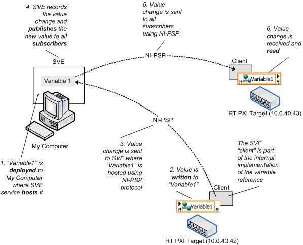
Figure 10. Shared Variable Engine and Network Shared Variable Value Changes
Network-Published Variables and LabVIEW Real-Time
You can enable real-time FIFOs with a network-published shared variable, but FIFO-enabled network-published shared variables have an important behavioral difference compared to real-time, FIFO-enabled, single-process shared variables. Recall that with the single-process shared variable, all writers and readers share a single, real-time FIFO; this is not the case with the network-published shared variable. Each reader of a network-published shared variable gets its own real-time FIFO in both the single-element and multielement cases, as shown below.
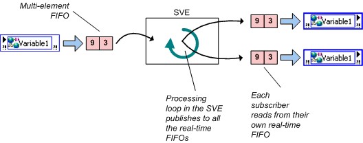
Figure 11. Real-Time FIFO-Enabled Network-Published Variable
Network Buffering
You can use buffering with the network-published shared variable. You can configure buffering in the Shared Variable Properties dialog box, as shown in Figure 12.
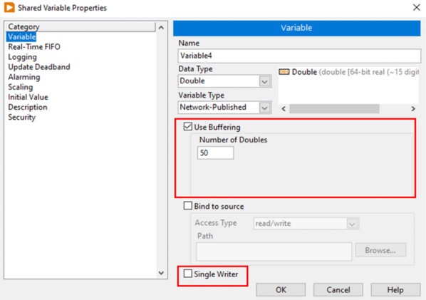
Figure 12. Enabling Buffering on a Networked-Published Shared Variable
With buffering enabled, you can specify the size of the buffer in units of the datatype, in this case, doubles.
With buffering, you can account for temporary fluctuations between read/write rates of a variable. Readers that occasionally read a variable slower than the writer can miss some updates. If the application can tolerate missing data points occasionally, the slower read rate does not affect the application and you do not need to enable buffering. However, if the reader must receive every update, enable buffering. You can set the size of the buffer on the Variable page of the Shared Variable Properties dialog box, so you can decide how many updates the application retains before it begins overwriting old data.
When you configure a network buffer in the dialog box above, you are actually configuring the size of two different buffers. The server side buffer, depicted as the buffer inside the box labeled Shared Variable Engine (SVE) in figure 13 below is automatically created and configured to be the same size as the client side buffer, more on that buffer in a minute. The client side buffer is more likely the one that you logically think of when you are configuring your shared variable to have buffering enabled. The client side buffer (depicted on the right hand side of figure 13) is the buffer responsible for maintaining the queue of previous values. It is this buffer that insulates your shared variables from fluctuations in loop speed or network traffic.
Unlike the real-time, FIFO-enabled, single-process variable, for which all writers and readers share the same real-time FIFO, each reader of a network-published shared variable gets its own buffer so readers do not interact with each other.
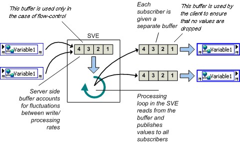
Figure 13. Buffering
Buffering helps only in situations in which the read/write rates have temporary fluctuations. If the application runs for an indefinite period of time, readers that always read at a slower rate than a writer eventually lose data regardless of the size of the buffer you specify. Because buffering allocates a buffer for every subscriber, to avoid unnecessary memory usage, use buffering only when necessary.
Network and Real-Time Buffering
If you enable both network buffering and the real-time FIFO, the implementation of the shared variable includes both a network buffer and a real-time FIFO. Recall that if the real-time FIFO is enabled, a new real-time FIFO is created for each writer and reader, which means that multiple writers and readers will not block each other.
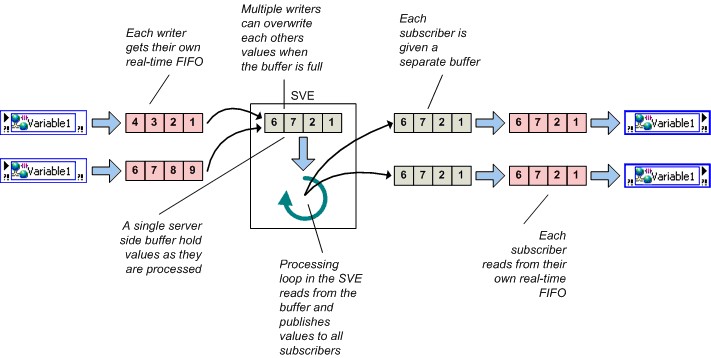
Figure 14. Network Buffering and Real-Time FIFOs
Although you can set the sizes of these two buffers independently, in most cases NI recommends that you keep them the same size. If you enable the real-time FIFO, LabVIEW creates a new real-time FIFO for each writer and reader. Therefore, multiple writers and readers do not block each other.
Buffer Lifetime
LabVIEW creates network and real-time FIFO buffers on an initial write or read, depending on the location of the buffers.
- Server-side buffers are created when a writer first writes to a shared variable.
- Client-side buffers are created when a subscription is established.
These occur when the VI containing the Shared Variable node starts. If a writer writes data to a shared variable before a given reader subscribes to that variable, the initial data values are not available to the subscriber.
Note: Prior to LabVIEW 8.6, creating buffers occurred when a Shared Variable read or write node was executed the first time.
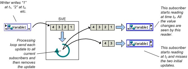
Figure 15. Buffer Lifetime
Buffer Overflow/Underflow
The network-published shared variable reports network buffer overflow and underflow conditions. The real-time FIFO in all versions will indicate FIFO overflow/underflow by returning errors.
Note: Legacy version of LabVIEW do not report network buffer overflow/underflow conditions. An application in LabVIEW 8.0 or 8.0.1 can check for network buffer underflows in two ways. Because the timestamp resolution of the shared variable is 1 ms, you can compare the timestamp of a shared variable to the subsequent read timestamp to detect buffer underflows when you update the variable at less than 1 kHz. Or the reader can use a sequence number bundled with the data to notice buffer overflows/underflows. You cannot use the second approach with shared variables used inside a time-critical loop if the data type is an array because the real-time FIFO-enabled shared variables do not support the Custom Control (cluster) data type if one of the elements of the cluster is an array.
Shared Variable Lifetime
As mentioned earlier, all shared variables are part of a project library. The SVE registers project libraries and the shared variables those libraries contain whenever LabVIEW needs one of those variables. By default, the SVE deploys and publishes a library of shared variables as soon as you run a VI that references any of the contained variables. Because the SVE deploys the entire library that owns a shared variable, the SVE publishes all shared variables in the library whether or not a running VI references them all. You can deploy any project library manually at any time by right-clicking the library in the Project Explorer window.
Stopping the VI or rebooting the machine that hosts the shared variable does not make the variable unavailable to the network. If you need to remove the shared variable from the network, you must explicitly undeploy the library the variable is part of in the Project Explorer window. You also can select Tools»Distributed System Manager to undeploy shared variables or entire project libraries of variables.
Note: Legacy Labview versions use the Variable Manager (Tools»Shared Variable»Variable Manager) instead of the Distributed System Manager to control shared variable deployment.
Front Panel Data Binding
An additional feature available for only network-published shared variables is front panel data binding. Drag a shared variable from the Project Explorer window to the front panel of a VI to create a control bound to the shared variable. When you enable data binding for a control, changing the value of the control changes the value of the shared variable to which the control is bound. While the VI is running, if the connection to the SVE is successful, a small green indicator appears next to the front panel object on the VI, as shown in Figure 16.
Figure 16. Binding a Front Panel Control to a Shared Variable
You can access and change the binding for any control or indicator on the Data Binding page of the Properties dialog box. When using the LabVIEW Real-Time Module or the LabVIEW DSC Module, you can select Tools»Shared Variable»Front Panel Binding Mass Configuration to display the Front Panel Binding Mass Configuration dialog box and create an operator interface that binds many controls and indicators to shared variables.
NI does not recommend using front panel data binding for applications that run on LabVIEW Real-Time because the front panel might not be present.
Programmatic Access
As discussed above, you can create, configure, and deploy shared variables interactively using the LabVIEW Project, and you can read from and write to shared variables using the shared variable node on the block diagram or through front panel data binding. In LabVIEW 2009 and later you also have programmatic access to all of this functionality.
Use VI Server to create project libraries and shared variables programmatically in applications where you need to create large numbers of shared variables. In addition, the LabVIEW DSC Module provides a comprehensive set of VIs to create and edit shared variables and project libraries programmatically as well as manage the SVE. You can create libraries of shared variables programmatically only on Windows systems; however, you can deploy these new libraries programmatically to Windows or LabVIEW Real-Time systems.
Use the programmatic Shared Variable API in applications where you need change dynamically the shared variable that a VI reads and writes, or where you need to read and write large numbers of variables. You can change a shared variable dynamically by building the URL programmatically.
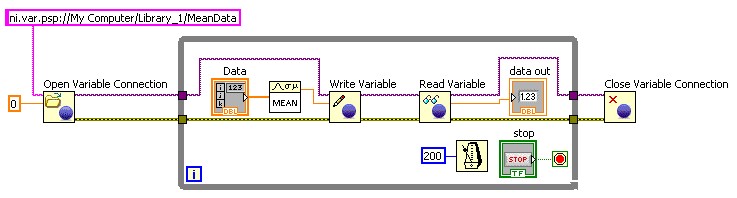
Figure 17. Using the programmatic Shared Variable API to Read and Write Shared Variables
In addition, with the Network Variable Library introducted in NI LabWindows/CVI 8.1 and NI Measurement Studio 8.1, you can read and write to shared variables in ANSI C, Visual Basic .NET or Visual C#.
The Shared Variable Engine
The SVE is a software framework that enables a networked-published shared variable to send values through the network. On Windows, LabVIEW configures the SVE as a service and launches the SVE at system startup. On a real-time target, the SVE is an installable startup component that loads when the system boots.
In order to use network-published shared variables, an SVE must be running on at least one of the nodes in the distributed system. Any node on the network can read or write to shared variables that the SVE publishes. As shown in Table 1, nodes can reference a variable without having the SVE installed. You also might have multiple SVEs installed on multiple systems simultaneously if you need to deploy shared variables in different locations based on application requirements.
Recommendations for Shared Variable Hosting Location
You must consider a number of factors when deciding from which computing device to deploy and host network-published shared variables you use in a distributed system.
Is the computing device compatible with SVE?
The following table summarizes the platforms for which the SVE is available and identifies the platforms that can use network-published shared variables through reference nodes or the DataSocket API. NI requires 32 MB of RAM and recommends 64 MB for the SVE on all applicable platforms.
Note that hosting of shared variables is still not supported on Linux nor Macintosh.
Windows PCs
| Mac OS
| Linux
| PXI
Real-Time | Compact FieldPoint
| CompactRIO
| Compact Vision System
| Commercial PCs with
LabVIEW Real-Time ETS | |
SVE
| X
| X
| ||||||
Reference Nodes
| X
| X
| ||||||
DataSocket API w/ PSP
|
Does the application require datalogging and supervisory functionality?
If you want to use the features of the LabVIEW DSC Module, you must host the shared variables on Windows. The LabVIEW DSC Module adds the following functionality to network-published shared variables:
· Historical logging to NI Citadel database.
· Networked alarms and alarm logging.
· Scaling.
· User-based security.
· Initial value.
· The ability to create custom I/O servers.
· Integration of the LabVIEW event structure with the shared variable.
· LabVIEW VIs to programmatically control all aspects of shared variables and the shared variable engine. These VIs are especially helpful for managing large numbers of shared variables.
Does the computing device have adequate processor and memory resources?
The SVE is an additional process that requires both processing and memory resources. In order to get the best performance in a distributed system, install the SVE on machines with the most memory and processing capabilities.
Which system is always online?
If you build a distributed application in which some of the systems might go offline periodically, host the SVE on a system that is always online.
Additional Features of the Shared Variable Engine
Figure 18 illustrates the many responsibilities of the SVE. In addition to managing networked-published shared variables, the SVE is responsible for:
· Collecting data received from I/O servers.
· Serving up data through the OPC and the PSP servers to subscribers.
· Providing scaling, alarming, and logging services for any shared variable with those services configured. These services are available only with the LabVIEW DSC Module.
· Monitoring for alarm conditions and responding accordingly.
I/O Servers
I/O servers are plug-ins to the SVE with which programs can use the SVE to publish data. NI FieldPoint includes an I/O server that publishes data directly from FieldPoint banks to the SVE. Because the SVE is an OPC server, the combination of the SVE and the FieldPoint I/O server serves as an FP OPC server. The FieldPoint installer does not include the SVE; it would have to be installed by another sofware component such as LabVIEW.
NI-DAQmx also includes an I/O server that can publish NI-DAQmx global virtual channels automatically to the SVE. This I/O server replaces the Traditional DAQ OPC server and RDA. NI-DAQmx includes the SVE and can install it when LabVIEW is not installed.
With the LabVIEW DSC Module, users can create new I/O servers.
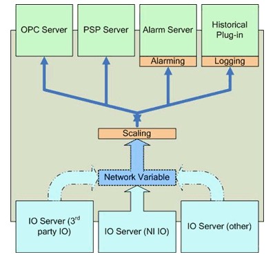
Figure 18. Shared Variable Engine (SVE)
OPC
The SVE is 3.0 compliant and can act as an OPC server on Windows machines. Any OPC client can write to or read from a shared variable hosted on a Windows machine. When you install the LabVIEW DSC Module on a Windows machine, the SVE also can act as an OPC client. You can bind shared variables that a Windows machine hosts to OPC data items with DSC and by writing to or reading from the variable to the OPC data item.
Because OPC is a technology based on COM, a Windows API, real-time targets do not work with OPC directly. As Figure 19 shows, you still can access OPC data items from a real-time target by hosting the shared variables on a Windows machine.
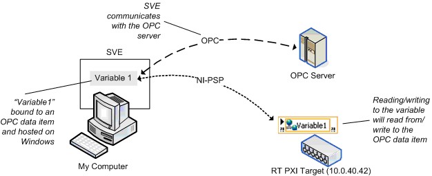
Figure 19. Binding to OPC Data Item
Performance
This section provides general guidelines for creating high-performing applications using the shared variable.
Because the single-process shared variable has an implementation similar to the LabVIEW global variables and real-time FIFOs, NI has no particular recommendations for achieving good performance for single-process shared variables. The following sections concentrate on the network-published shared variable.
Share the Processor
The network-published shared variable simplifies LabVIEW block diagrams by hiding many of the implementation details of network programming. Applications consist of LabVIEW VIs as well as the SVE and the SVE client code. In order to get the best shared variable performance, develop the application so that it relinquishes the processor regularly for the SVE threads to run. One way to accomplish this is to place waits in the processing loops and ensure that the application does not use untimed loops. The exact amount of time you must wait is application, processor, and network-dependent; every application requires some level of empirical tuning in order to achieve the best performance.
Consider the Location of the SVE
The Recommendations for Shared Variable Hosting Location section discussed a number of factors you must consider when deciding where to install the SVE. Figure 20 shows another factor that can greatly impact the performance of the shared variable. This example involves a real-time target, but the basic principles also apply to nonreal-time systems. Figure 20 shows an inefficient use of network-published shared variables: you generate data on a real-time target and need to log the data processed locally and monitor it from a remote machine. Because variable subscribers must receive data from the SVE, the latency between the write in the high-priority loop and the read in the normal-priority loop is large and involves two trips across the network.
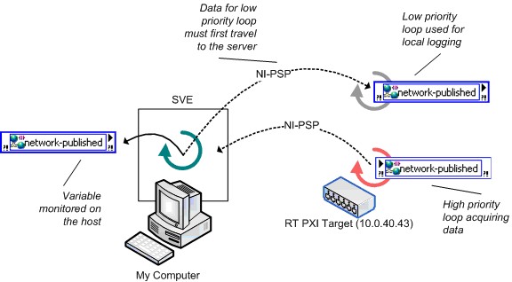
Figure 20. Inefficient Use of Network-Published Variables on Real-Time
Figure 21 shows a better architecture for this application. The application uses a single-process shared variable to transfer data between the high-priority loop and the low-priority loop, reducing the latency greatly. The low-priority loop logs the data and writes the update to a network-published shared variable for the subscriber at the host.
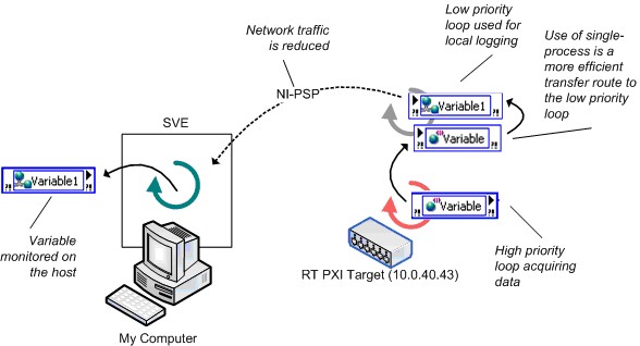
Figure 21. Efficient Use of Network-Published Variables on Real-Time
Benchmarks
This section compares the performance of the shared variable to other applicable data sharing methods in LabVIEW, such as the LabVIEW global variable, real-time FIFOs, and TCP/IP. The following table summarizes the tests discussed are presented in the following sections.
Test | Description | SVE Location | Notes |
|---|---|---|---|
T1 | Single-process shared variable vs. global variable | N/A | Establish maximum read/write rates. |
T2 | Single-process shared variable w/ real-time FIFO vs. real-time FIFO VIs | N/A | Establish maximum read/write rates when using real-time FIFOs. Determine the highest sustainable rate at which you can write to a shared variable or real-time FIFO in a timed loop and simultaneously read the data back from a normal priority loop. |
T3 | Network-published shared variable w/ real-time FIFO vs. 2-loop real-time FIFO w/ TCP | PXI running LV RT | Establish the maximum rate single-point data can be streamed across the network. Shared variable: reader VI is always on the host.RT-FIFO + TCP: similar to T2 with the addition of TCP communication./IP networking. |
T4 | Network-published shared variable footprint | RT Series Target | Establish memory usage of shared variables after deployment. |
T5 | Comparison between 8.2 Nework-published shared variables and 8.5 variables - streaming | RT Series Target | Comparing the new 8.5 implementation of NI-PSP to the 8.20 and earlier implementation. This benchmark measures throughput of an application streaming waveform data from a cRIO device to a desktop host. |
T6 | Comparison between 8.2 Nework-published shared variables and 8.5 variables - high channel count | RT Series Target | Comparing the new 8.5 implementation of NI-PSP to the 8.20 and earlier implementation. This benchmark measures throughput of a high channel count application on a cRIO device. |
Table 2. Benchmark Overview
The following sections describe the code NI created for each of the benchmarks, followed with the actual benchmark results. The Methodology and Configuration section discusses in greater detail the chosen methodology for each benchmark and the detailed configuration used for the hardware and software on which the benchmark was run.
Single-Process Shared Variables vs. LabVIEW Global Variables
The single-process shared variable is similar to the LabVIEW global variable. In fact, the implementation of the single-process shared variable is a LabVIEW global with the added time-stamping functionality.
To compare the performance of the single-process shared variable to the LabVIEW global variable, NI created benchmark VIs to measure the number of times the VI can read and write to a LabVIEW global variable or single-process shared variable every second. Figure 22 shows the single-process shared variable read benchmark. The single-process shared variable write benchmark and the LabVIEW global read/write benchmarks follow the same pattern.
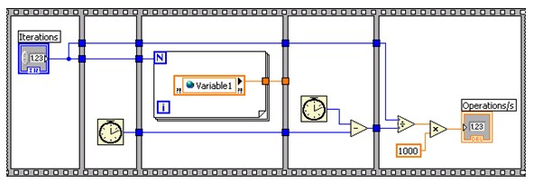
Figure 22. Single-Process Shared Variable Read Benchmarking VI
The combination read/write test also includes code to validate that every point written also can be read back in the same iteration of the loop with no data corruption.
T1 Test Results
Figure 23 shows the results of Test T1. The results show that the read performance for a single-process shared variable is lower than the read performance for a LabVIEW global variable. The write performance, and hence the read/write performance, of the single-process shared variable is slightly lower than that of the LabVIEW global variable. Performance of single-process shared variables will be affected by enabling and disabling the timestamp functionality, so it is recommended to turn the timestamp off if it is not useful.
The Methodology and Configuration section explains the specific benchmarking methodology and configuration details for this test set.
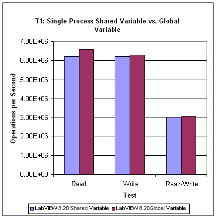
Figure 23. Single-Process Shared Variable vs. Global Variable Performance
Single-Process Shared Variables vs. Real-Time FIFOs
NI benchmarked sustainable throughput to compare the performance of the FIFO-enabled single-process shared variable against traditional real-time FIFO VIs. The benchmark also examines the effect of the size of the transferred data, or payload, for each of the two real-time FIFO implementations.
The tests consist of a time-critical loop (TCL) generating data and a normal-priority loop (NPL) consuming the data. NI determined the effect of the payload size by sweeping through a range of double-precision scalar and array data types. The scalar type determines the throughput when the payload is one double, and the array types determine the throughput for the rest of the payloads. The test records the maximum sustainable throughput by determining the maximum sustainable speed at which you can execute both loops with no data loss.
Figure 24 shows a simplified diagram of the real-time FIFO benchmark that omits much of the necessary code required to create and destroy the FIFOs. Note that as of LabVIEW 8.20, a new FIFO function was introduced to replace the FIFO SubVI's shown here. The FIFO functions were used for the data graphed in this paper, and perform better than their 8.0.x SubVI predecessors.
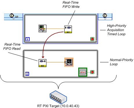
Figure 24. Simplified Real-Time FIFO Benchmarking VI
An equivalent version of the test uses the single-process shared variable. Figure 25 shows a simplified depiction of that diagram.
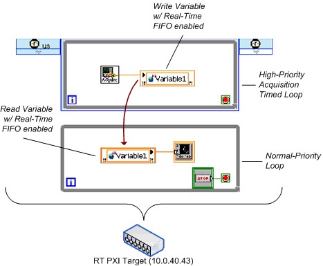
Figure 25. Simplified FIFO-Enabled Single-Process Shared Variable Benchmarking VI
T2 Test Results
Figure 26 and 27 shows the results of Test T2, comparing the performance of the FIFO-enabled single-process shared variable against real-time FIFO functions. The results indicate that using the single-process shared variable is marginally slower than using real-time FIFOs.
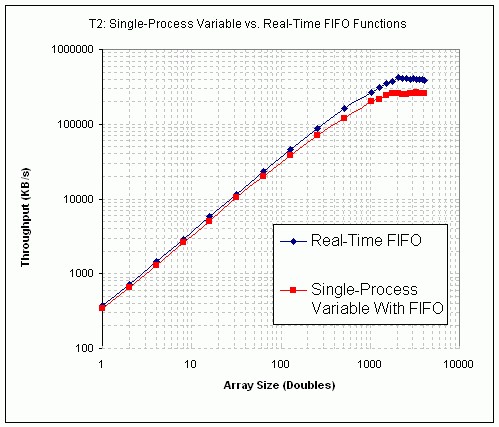
Figure 26. Single-Process Shared Variable vs. Real-Time FIFO VI Performance (PXI)
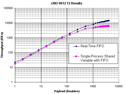
Figure 27. Single-Process Shared Variable vs. Real-Time FIFO VI Performance (cRIO 9012)
Network-Published Shared Variables vs. Real-Time FIFOs and TCP/IP
With the flexibility of the shared variable, you can publish a single-process shared variable quickly across the network with just a few configuration changes. For real-time applications in particular, performing the same transformation in earlier versions of LabVIEW requires the introduction of a large amount of code to read the real-time FIFOs on the RT Series controller and then send the data over the network using one of the many available networking protocols. To compare the performance of these two different approaches, NI again created benchmark VIs to measure the sustainable throughput of each with no data loss across a range of payloads.
For the prevariable approach, the benchmark VI uses real-time FIFOs and TCP/IP. A TCL generates data and places it in a real-time FIFO; an NPL reads the data out of the FIFO and sends it over the network using TCP/IP. A host PC receives the data and validates that no data loss occurs.
Figure 28 shows a simplified diagram of the real-time FIFO and TCP/IP benchmark. Again, this diagram vastly simplifies the actual benchmark VI.
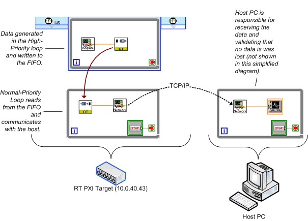
Figure 28. Simplified Real-Time FIFO and TCP/IP Benchmarking VI
NI created an equivalent version of the test using the network-published shared variable. Figure 29 shows a simplified diagram.
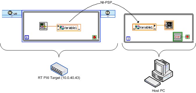
Figure 29. Simplified Real-Time FIFO-Enabled Network-Published Shared Variable Benchmarking VI
T3 Test Results
This section contains the results of Test T3, comparing the performance of the real-time FIFO-enabled network-published shared variable to that of equivalent code relying on real-time FIFO VIs and LabVIEW TCP/IP primitives. Figure 30 shows the results when the LabVIEW Real-Time target is an embedded RT Series PXI controller.
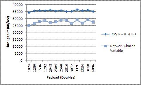
Figure 30. Network-Published Shared Variable vs. Real-Time FIFO and TCP VI Performance (PXI)
T3 Results indicate that throughput of Network-published Shared Variables approaches that of TCP and that both are consistent across moderate to large payload sizes. The shared variable makes your programming job easier, but that does not come without a cost. It should be noted, however, that if a naive TCP implementation is used, it could be easy to underperform shared variables, particularly with the new 8.5 implementation of NI-PSP.
T4 Test Results
Memory Footprint of the Network-Published Shared Variable
Note that no significant changes to variable footprint have been made in LabVIEW 8.5. Therefore, this benchmark was not rerun.
Determining the memory footprint of the shared variable is difficult because the memory used by the shared variable depends on the configuration. Network-published shared variables with buffering, for example, allocate memory dynamically as needed by the program. Configuring a shared variable to use real-time FIFOs also increases memory usage because in addition to network buffers, LabVIEW creates buffers for the FIFO. Therefore the benchmark results in this paper provide only a baseline measurement of memory.
Figure 31 shows the memory that the SVE uses after LabVIEW deploys 500 and 1000 shared variables of the specified types to it. The graph shows that the type of variable does not affect the memory usage of the deployed shared variables significantly. Note that these are nonbuffered variables.
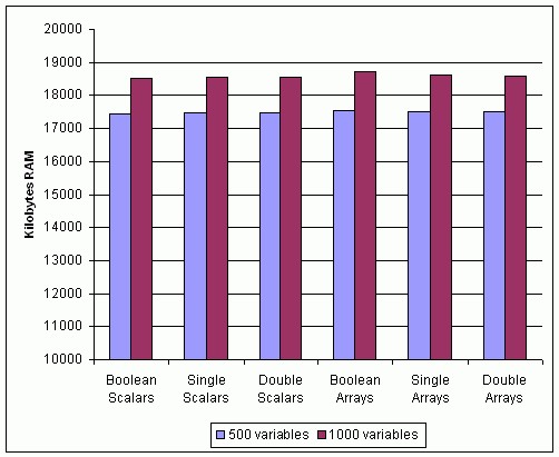
Figure 31. Memory Usage of Network-Published Shared Variables with Different Data Types
Figure 32 shows memory usage as a function of the number of shared variables deployed. This test uses only one type of variable, an empty Boolean array. The memory usage increases linearly with the variable count.
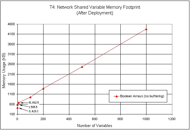
Figure 32. Memory Usage of Shared Variables of Different Sizes
T5 Test Results
Comparison between 8.2 Nework-published shared variables and 8.5 variables - streaming
In LabVIEW 8.5, we have reimplemented the bottom layer of the network protocol used to transport shared variable data. It offers significantly better performance.
In this case, we hosted a single variable of type Waveform of Doubles on a cRIO 9012. We generated all the data, then in a tight loop, transferred the data to the host which read it out of another waveform shared variable node as fast as it could.
You can see from figure 30, that performance has improved in LabVIEW 8.5 by over 600% for this use case.
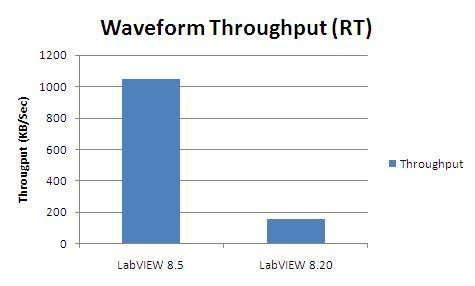
Figure 33. Waveform throughput comparison between LabVIEW 8.5 and LabVIEW 8.20 (and earlier)
T6 Test Results
Comparison between 8.2 Nework-published shared variables and 8.5 variables - streaming
In this test, we used the same two targets as in T5, but instead of transferring a single variable, we changed the datatype to a double and varied the number of shared variables from 1 - 1000, measuring throughput along the way. Again, all the variables were hosted on the cRIO 9012, incrementing data was generated there as well and transmitted to the host where they were read.
Figure 34 again shows a significant performance increase from LabVIEW 8.20 to LabVIEW 8.5. However, the throughput is significantly less in the case of many smaller variables than it is for a single large variable as in T5. This is because each variable has associated with it a fixed amount of overhead. When many variables are used, this overhead is multiplied by the nubmer of variables and becomes quite noticable.
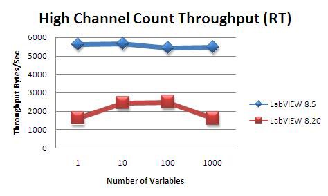
Figure 34. High channel count throughput comparison between LabVIEW 8.5 and LabVIEW 8.20 (and earlier)
Methodology and Configuration
This section provides detailed information regarding the benchmarking process for all the previously mentioned test sets.
T1 Methodology and Considerations
Test T1 uses a simple benchmarking template to determine read and write rates through simple averaging over a large number of iterations. Each test executed a total of 500 million iterations for total execution times in the order of one minute, timed with millisecond resolution.
T1 Hardware/Software Configuration
Host Hardware
- Dell Precision 450
- Dual Intel Xeon 2.4 GHz Pentium-class processors
- 1 GB DRAM
Host Software
- Windows XP SP2
- LabVIEW 8.20
T2 Methodology and Considerations
Test T2 measures throughput by identifying the maximum sustainable communication rate between tasks running at different priorities. A timed loop running with microsecond resolution contains the data producer. The consumer of the data is a free-running, normal-priority loop that reads from the real-time FIFO or single-process shared variable until empty, repeating this process until a certain amount of time elapses without errors. The test result is valid only if all of the following statements are true:
- No buffer overflows occur
- Data integrity is preserved: no data losses occur and the consumer receives the data in the order it was sent
- Timed loop is able to keep up after a designated warm-up period of 1 s
The single-process shared variable receiver loop performs simple data integrity checks, such as ensuring that the expected number of data points were received and that the received message pattern does not lack intermediate values.
NI configured the buffer sizes for the real-time FIFO and shared variable FIFO buffers to be 100 elements deep for all test variations and data types involved.
T2 Hardware/Software Configuration
PXI Hardware
- NI PXI-8196 RT Series controller
- 2.0 GHz Pentium-class processor
- 256 MB DRAM
- Broadcom 57xx (1 Gb/s built-in Ethernet adapter)
PXI Software
- LabVIEW 8.20 Real-Time Module
- Network Variable Engine 1.2.0
- Variable Client Support 1.2.0
- Broadcom 57xx Gigabit Ethernet driver 2.1 configured in polling mode
CompactRIO Hardware
- NI cRIO 9012 controller
- 400 MHz processor
- 64 MB DRAM
CompactRIO Software
- LabVIEW 8.20 Real-Time Module
- Network Variable Engine 1.2.0
- Variable Client Support 1.2.0
T3 Methodology and Considerations
Test T3 measures throughput directly by recording the amount of data transmitted over the network and the overall duration of the test. A timed loop running with microsecond resolution contains the data producer, which is responsible for writing a specific data pattern to the network-published shared variable or real-time FIFO VIs.
For the network-published shared variable case, an NPL runs on the host system and reads from the variable in a free-running while loop. For the real-time FIFO VI test, the NPL runs on the real-time system, checking the state of the FIFO at a given rate, reading all available data, and sending it over the network using TCP. The benchmark results show the effect of having this polling period set to either 1 or 10 ms.
The test result is valid only if all of the following statements are true:
- No buffer overflows occur, neither FIFO nor network
- Data integrity is preserved: no data losses occur and the consumer receives the data in the order it was sent
- The timed loop in the TCL VI is able to keep up after a designated warm-up period of 1 s
After reading each data point, the NPL for the network variable test checks the data pattern for correctness. For the real-time FIFO test, the TCL is responsible for validation based on whether a real-time FIFO overflow occurred.
To help avoid data loss, NI configured the buffer sizes to be no smaller than the ratio between the NPL and TCL loop periods, with a lower bound of 100 elements as the minimum size for the real-time FIFO buffers.
T3 Hardware/Software Configuration
Host Hardware
- Intel Core 2 Duo 1.8 GHz
- 2 GB DRAM
- Intel PRO/1000 (1 Gb/s Ethernet adapter)
Host Software
- Windows Vista 64
- LabVIEW 8
Network Configuration
1Gb/s switched network
PXI Hardware
- NI PXI-8196 RT controller
- 2.0 GHz Pentium-class processor
- 256 MB DRAM
- Broadcom 57xx (1 Gb/s built-in Ethernet adapter)
PXI Software
- LabVIEW 8.5 Real-Time Module
- Network Variable Engine 1.2.0
- Variable Client Support 1.2.0
- Broadcom 57xx Gigabit Ethernet driver 2.1
T4 Methodology and Considerations
In Test T4, NI used nonbuffered, network-published shared variables with the following data types: double, single, Boolean, double array, single array, and Boolean array.
T4 Hardware/Software Configuration
PXI Hardware
- NI PXI-8196 RT Controller
- 2.0 GHz Pentium-class processor
- 256 MB DRAM
- Broadcom 57xx (1 Gb/s built-in Ethernet adapter)
PXI Software
- LabVIEW Real-Time Module 8.0
- Network Variable Engine 1.0.0
- Variable Client Support 1.0.0
- Broadcom 57xx Gigabit Ethernet driver 1.0.1.3.0
T5 and T6 Methodology and Considerations
In test T5 and T6, NI used nonbuffered, network-published shared variables of the Waveform of Double datatype.
T5 and T6 Hardware/Software Configuration
Host Hardware
- 64 Bit Intel Core 2 Duo 1.8 GHz
- 2 GB RAM
- Gigabit ethernet
Host Software
- Windows Vista 64
- LabVIEW 8.20 and LabVIEW 8.5
CompactRIO Hardware
- cRIO 9012
- 64 MB RAM
CompactRIO Software
- LabVIEW RT 8.20 and LabVIEW RT 8.5
- Network Variable Engine 1.2 (with LabVIEW 8.20) and 1.4 (with LabVIEW 8.5)
- Variable Client Support 1.0 (with LabVIEW 8.20) and 1.4 (with LabVIEW 8.5)