From Friday, April 19th (11:00 PM CDT) through Saturday, April 20th (2:00 PM CDT), 2024, ni.com will undergo system upgrades that may result in temporary service interruption.
We appreciate your patience as we improve our online experience.
From Friday, April 19th (11:00 PM CDT) through Saturday, April 20th (2:00 PM CDT), 2024, ni.com will undergo system upgrades that may result in temporary service interruption.
We appreciate your patience as we improve our online experience.
As the usage of digital measurement instruments during the test and measurement process increases, acquiring large quantities of data becomes easier. However, the methods of processing and extracting useful information from the acquired data become a challenge.
During the test and measurement process, you often see a mathematical relationship between observed values and independent variables, such as the relationship between temperature measurements, an observable value, and measurement error, an independent variable that results from an inaccurate measuring device. One way to find the mathematical relationship is curve fitting, which defines an appropriate curve to fit the observed values and uses a curve function to analyze the relationship between the variables.
You can use curve fitting to perform the following tasks:
This document describes the different curve fitting models, methods, and the LabVIEW VIs you can use to perform curve fitting.
The purpose of curve fitting is to find a function f(x) in a function class Φ for the data (xi, yi) where i=0, 1, 2,…, n–1. The function f(x) minimizes the residual under the weight W. The residual is the distance between the data samples and f(x). A smaller residual means a better fit. In geometry, curve fitting is a curve y=f(x) that fits the data (xi, yi) where i=0, 1, 2,…, n–1.
In LabVIEW, you can use the following VIs to calculate the curve fitting function.
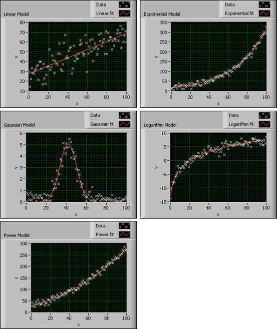
These VIs create different types of curve fitting models for the data set. Refer to the LabVIEW Help for information about using these VIs. The following graphs show the different types of fitting models you can create with LabVIEW.
Figure 1. Curve Fitting Models in LabVIEW
Before fitting the data set, you must decide which fitting model to use. An improper choice, for example, using a linear model to fit logarithmic data, leads to an incorrect fitting result or a result that inaccurately determines the characteristics of the data set. Therefore, you first must choose an appropriate fitting model based on the data distribution shape, and then judge if the model is suitable according to the result.
Every fitting model VI in LabVIEW has a Weight input. The Weight input default is 1, which means all data samples have the same influence on the fitting result. In some cases, outliers exist in the data set due to external factors such as noise. If you calculate the outliers at the same weight as the data samples, you risk a negative effect on the fitting result. Therefore, you can adjust the weight of the outliers, even set the weight to 0, to eliminate the negative influence.
You also can use the Curve Fitting Express VI in LabVIEW to develop a curve fitting application.
Different fitting methods can evaluate the input data to find the curve fitting model parameters. Each method has its own criteria for evaluating the fitting residual in finding the fitted curve. By understanding the criteria for each method, you can choose the most appropriate method to apply to the data set and fit the curve. In LabVIEW, you can apply the Least Square (LS), Least Absolute Residual (LAR), or Bisquare fitting method to the Linear Fit, Exponential Fit, Power Fit, Gaussian Peak Fit, or Logarithm Fit VI to find the function f(x).
The LS method finds f(x) by minimizing the residual according to the following formula:
where n is the number of data samples
wi is the ith element of the array of weights for the data samples
f(xi) is the ith element of the array of y-values of the fitted model
yi is the ith element of the data set (xi, yi)
The LAR method finds f(x) by minimizing the residual according to the following formula:
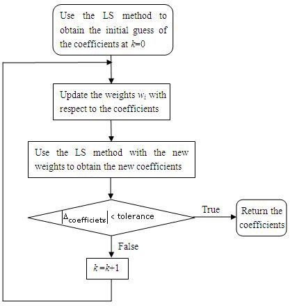
The Bisquare method finds f(x) by using an iterative process, as shown in the following flowchart, and calculates the residual by using the same formula as in the LS method. The Bisquare method calculates the data starting from iteration k.
Figure 2. Bisquare Method Flowchart
Because the LS, LAR, and Bisquare methods calculate f(x) differently, you want to choose the curve fitting method depending on the data set. For example, the LAR and Bisquare fitting methods are robust fitting methods. Use these methods if outliers exist in the data set. The following sections describe the LS, LAR, and Bisquare calculation methods in detail.
The least square method begins with a linear equations solution.
Ax = b
A is a matrix and x and b are vectors. Ax–b represents the error of the equations.
The following equation represents the square of the error of the previous equation.
E(x) = (Ax-b)T(Ax-b) = xTATAx-2bTAx+bTb
To minimize the square error E(x), calculate the derivative of the previous function and set the result to zero:
E’(x) = 0
2ATAx-2ATb = 0
ATAx =ATb
x = (ATA)-1ATb
From the algorithm flow, you can see the efficiency of the calculation process, because the process is not iterative. Applications demanding efficiency can use this calculation process.
The LS method calculates x by minimizing the square error and processing data that has Gaussian-distributed noise. If the noise is not Gaussian-distributed, for example, if the data contains outliers, the LS method is not suitable. You can use another method, such as the LAR or Bisquare method, to process data containing non-Gaussian-distributed noise.
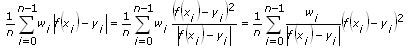
The LAR method minimizes the residual according to the following formula:
From the formula, you can see that the LAR method is an LS method with changing weights. If the data sample is far from f(x), the weight is set relatively lower after each iteration so that this data sample has less negative influence on the fitting result. Therefore, the LAR method is suitable for data with outliers.
Like the LAR method, the Bisquare method also uses iteration to modify the weights of data samples. In most cases, the Bisquare method is less sensitive to outliers than the LAR method.
If you compare the three curve fitting methods, the LAR and Bisquare methods decrease the influence of outliers by adjusting the weight of each data sample using an iterative process. Unfortunately, adjusting the weight of each data sample also decreases the efficiency of the LAR and Bisquare methods.
To better compare the three methods, examine the following experiment. Use the three methods to fit the same data set: a linear model containing 50 data samples with noise. The following table shows the computation times for each method:
Table 1. Processing Times for Three Fitting Methods
| Fitting method | LS | LAR | Bisquare |
| Time(μs) | 3.5 | 30 | 60 |
As you can see from the previous table, the LS method has the highest efficiency.
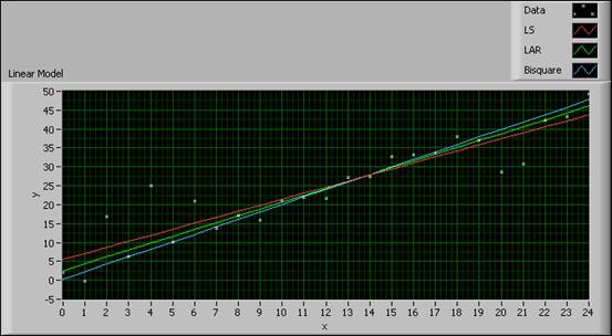
The following figure shows the influence of outliers on the three methods:
Figure 3. Comparison among Three Fitting Methods
The data samples far from the fitted curves are outliers. In the previous figure, you can regard the data samples at (2, 17), (20, 29), and (21, 31) as outliers. The results indicate the outliers have a greater influence on the LS method than on the LAR and Bisquare methods.
From the previous experiment, you can see that when choosing an appropriate fitting method, you must take both data quality and calculation efficiency into consideration.
In addition to the Linear Fit, Exponential Fit, Gaussian Peak Fit, Logarithm Fit, and Power Fit VIs, you also can use the following VIs to calculate the curve fitting function.
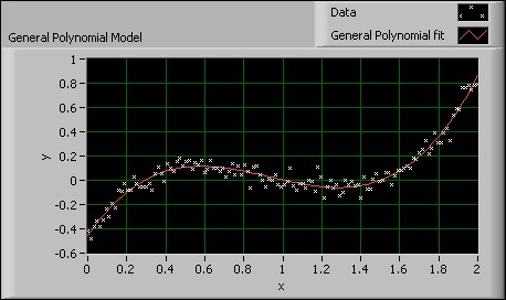
The General Polynomial Fit VI fits the data set to a polynomial function of the general form:
f(x) = a + bx + cx2 + …
The following figure shows a General Polynomial curve fit using a third order polynomial to find the real zeroes of a data set. You can see that the zeroes occur at approximately (0.3, 0), (1, 0), and (1.5, 0).
Figure 4. General Polynomial Model
This VI calculates the mean square error (MSE) using the following equation:
When you use the General Polynomial Fit VI, you first need to set the Polynomial Order input. A high Polynomial Order does not guarantee a better fitting result and can cause oscillation. A tenth order polynomial or lower can satisfy most applications. The Polynomial Order default is 2.
This VI has a Coefficient Constraint input. You can set this input if you know the exact values of the polynomial coefficients. By setting this input, the VI calculates a result closer to the true value.
The General Linear Fit VI fits the data set according to the following equation:
y = a0 + a1f1(x) + a2f2(x) + …+ak-1fk-1(x)
where y is a linear combination of the coefficients a0, a1, a2, …, ak-1 and k is the number of coefficients.
The following equations show you how to extend the concept of a linear combination of coefficients so that the multiplier for a1 is some function of x.
y = a0 + a1sin(ωx)
y = a0 + a1x2
y = a0 + a1cos(ωx2)
where ω is the angular frequency.
In each of the previous equations, y is a linear combination of the coefficients a0 and a1. For the General Linear Fit VI, y also can be a linear combination of several coefficients. Each coefficient has a multiplier of some function of x. Therefore, you can use the General Linear Fit VI to calculate and represent the coefficients of the functional models as linear combinations of the coefficients.
y = a0 + a1sin(ωx)
y = a0 + a1x2 + a2cos(ωx2)
y = a0 + a1(3sin(ωx)) + a2x3 + (a3/x) + …
In each of the previous equations, y can be both a linear function of the coefficients a0, a1, a2,…, and a nonlinear function of x.
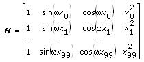
When you use the General Linear Fit VI, you must build the observation matrix H. For example, the following equation defines a model using data from a transducer.
y = a0 + a1sin(ωx) + a2cos(ωx) + a3x2
The following table shows the multipliers for the coefficients, aj, in the previous equation.
|
Coefficient |
Multiplier |
|
ao |
1 |
|
a1 |
sin(ωx) |
|
a2 |
cos(ωx) |
|
a3 |
x2 |
To build the observation matrix H, each column value in H equals the independent function, or multiplier, evaluated at each x value, xi. The following equation defines the observation matrix H for a data set containing 100 x values using the previous equation.
If the data set contains n data points and k coefficients for the coefficient a0, a1, …, ak– 1, then H is an n × k observation matrix. Therefore, the number of rows in H equals the number of data points, n. The number of columns in H equals the number of coefficients, k.
To obtain the coefficients, a0, a1, …, ak – 1, the General Linear Fit VI solves the following linear equation:
H a = y
where a = [a0 a1 … ak – 1]T and y = [y0 y1 … yn – 1]T.
A spline is a piecewise polynomial function for interpolating and smoothing. In curve fitting, splines approximate complex shapes.
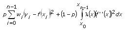
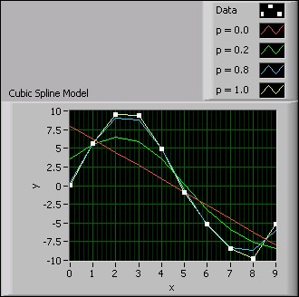
The Cubic Spline Fit VI fits the data set (xi, yi) by minimizing the following function:
where p is the balance parameter
wi is the ith element of the array of weights for the data set
yi is the ith element of the data set (xi, yi)
xi is the ith element of the data set (xi, yi)
f"(x) is the second order derivative of the cubic spline function, f(x)
λ(x) is the piecewise constant function:
where λi is the ith element of the Smoothness input of the VI.
If the Balance Parameter input p is 0, the cubic spline model is equivalent to a linear model. If the Balance Parameter input p is 1, the fitting method is equivalent to cubic spline interpolation. p must fall in the range [0, 1] to make the fitted curve both close to the observations and smooth. The closer p is to 0, the smoother the fitted curve. The closer p is to 1, the closer the fitted curve is to the observations. The following figure shows the fitting results when p takes different values.
Figure 5. Cubic Spline Model
You can see from the previous figure that when p equals 1.0, the fitted curve is closest to the observation data. When p equals 0.0, the fitted curve is the smoothest, but the curve does not intercept at any data points.
The Nonlinear Curve Fit VI fits data to the curve using the nonlinear Levenberg-Marquardt method according to the following equation:
y = f(x; a0, a1, a2, …, ak)
where a0, a1, a2, …, ak are the coefficients and k is the number of coefficients.
The nonlinear Levenberg-Marquardt method is the most general curve fitting method and does not require y to have a linear relationship with a0, a1, a2, …, ak. You can use the nonlinear Levenberg-Marquardt method to fit linear or nonlinear curves. However, the most common application of the method is to fit a nonlinear curve, because the general linear fit method is better for linear curve fitting.
LabVIEW also provides the Constrained Nonlinear Curve Fit VI to fit a nonlinear curve with constraints. You can set the upper and lower limits of each fitting parameter based on prior knowledge about the data set to obtain a better fitting result.
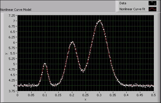
The following figure shows the use of the Nonlinear Curve Fit VI on a data set. The nonlinear nature of the data set is appropriate for applying the Levenberg-Marquardt method.
Figure 6. Nonlinear Curve Model
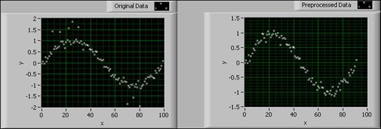
The Remove Outliers VI preprocesses the data set by removing data points that fall outside of a range. The VI eliminates the influence of outliers on the objective function. The following figure shows a data set before and after the application of the Remove Outliers VI.
Figure 7. Remove Outliers VI
In the previous figure, the graph on the left shows the original data set with the existence of outliers. The graph on the right shows the preprocessed data after removing the outliers.
You also can remove the outliers that fall within the array indices you specify.
Some data sets demand a higher degree of preprocessing. A median filter preprocessing tool is useful for both removing the outliers and smoothing out data.
LabVIEW offers VIs to evaluate the data results after performing curve fitting. These VIs can determine the accuracy of the curve fitting results and calculate the confidence and prediction intervals in a series of measurements.
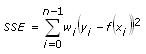
The Goodness of Fit VI evaluates the fitting result and calculates the sum of squares error (SSE), R-square error (R2), and root mean squared error (RMSE) based on the fitting result. These three statistical parameters describe how well the fitted model matches the original data set. The following equations describe the SSE and RMSE, respectively.
where DOF is the degree of freedom.
The SSE and RMSE reflect the influence of random factors and show the difference between the data set and the fitted model.
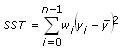
The following equation describes R-square:
where SST is the total sum of squares according to the following equation:
R-square is a quantitative representation of the fitting level. A high R-square means a better fit between the fitting model and the data set. Because R-square is a fractional representation of the SSE and SST, the value must be between 0 and 1.
0 ≤ R-square ≤ 1
When the data samples exactly fit on the fitted curve, SSE equals 0 and R-square equals 1. When some of the data samples are outside of the fitted curve, SSE is greater than 0 and R-square is less than 1. Because R-square is normalized, the closer the R-square is to 1, the higher the fitting level and the less smooth the curve.
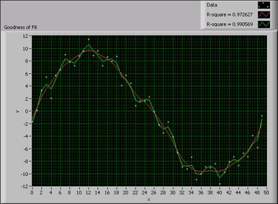
The following figure shows the fitted curves of a data set with different R-square results.
Figure 8. Fitting Results with Different R-Square Values
You can see from the previous figure that the fitted curve with R-square equal to 0.99 fits the data set more closely but is less smooth than the fitted curve with R-square equal to 0.97.
In the real-world testing and measurement process, as data samples from each experiment in a series of experiments differ due to measurement error, the fitting results also differ. For example, if the measurement error does not correlate and distributes normally among all experiments, you can use the confidence interval to estimate the uncertainty of the fitting parameters. You also can use the prediction interval to estimate the uncertainty of the dependent values of the data set.
For example, you have the sample set (x0, y0), (x1, y1), …, (xn-1, yn-1) for the linear fit function y = a0x + a1. For each data sample, (xi, yi), the variance of the measurement error,, is specified by the weight,
You can use the function form x = (ATA)-1ATb of the LS method to fit the data according to the following equation.
where a = [a0 a1]T
y = [y0 y1 … yn-1]T
You can rewrite the covariance matrix of parameters, a0 and a1, as the following equation.
where J is the Jacobean matrix
m is the number of parameters
n is the number of data samples
In the previous equation, the number of parameters, m, equals 2. The ith diagonal element of C, Cii, is the variance of the parameter ai, .
The confidence interval estimates the uncertainty of the fitting parameters at a certain confidence level . For example, a 95% confidence interval means that the true value of the fitting parameter has a 95% probability of falling within the confidence interval. The confidence interval of the ith fitting parameter is:
where is the Student’s t inverse cumulative distribution function of n–m degrees of freedom at probability
and
is the standard deviation of the parameter ai and equals
.
You also can estimate the confidence interval of each data sample at a certain confidence level . For example, a 95% confidence interval of a sample means that the true value of the sample has a 95% probability of falling within the confidence interval. The confidence interval of the ith data sample is:
where diagi(A) denotes the ith diagonal element of matrix A. In the above formula, the matrix (JCJ)T represents matrix A.
The prediction interval estimates the uncertainty of the data samples in the subsequent measurement experiment at a certain confidence level . For example, a 95% prediction interval means that the data sample has a 95% probability of falling within the prediction interval in the next measurement experiment. Because the prediction interval reflects not only the uncertainty of the true value, but also the uncertainty of the next measurement, the prediction interval is wider than the confidence interval. The prediction interval of the ith sample is:
LabVIEW provides VIs to calculate the confidence interval and prediction interval of the common curve fitting models, such as the linear fit, exponential fit, Gaussian peak fit, logarithm fit, and power fit models. These VIs calculate the upper and lower bounds of the confidence interval or prediction interval according to the confidence level you set.
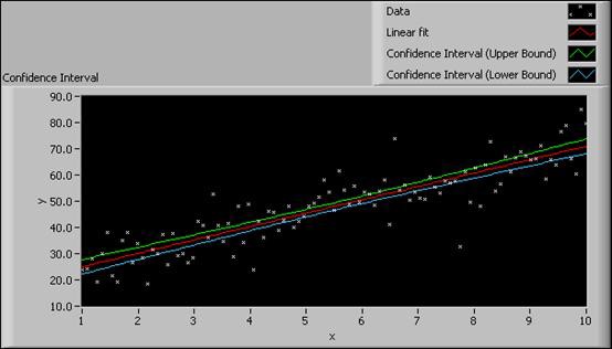
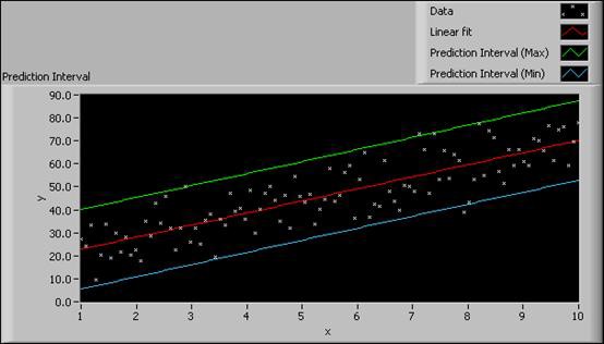
The following figure shows examples of the Confidence Interval graph and the Prediction Interval graph, respectively, for the same data set.
Figure 9. Confidence Interval and Prediction Interval
From the Confidence Interval graph, you can see that the confidence interval is narrow. A small confidence interval indicates a fitted curve that is close to the real curve. From the Prediction Interval graph, you can conclude that each data sample in the next measurement experiment will have a 95% chance of falling within the prediction interval.
As measurement and data acquisition instruments increase in age, the measurement errors which affect data precision also increase. In order to ensure accurate measurement results, you can use the curve fitting method to find the error function to compensate for data errors.
For example, examine an experiment in which a thermometer measures the temperature between –50ºC and 90ºC. Suppose T1 is the measured temperature, T2 is the ambient temperature, and Te is the measurement error where Te is T1 minus T2. By measuring different temperatures within the measureable range of –50ºC and 90ºC, you obtain the following data table:
Table 2. Ambient Temperature and Measured Temperature Readings
|
Ambient Temperature |
Measured Temperature | Ambient Temperature | Measured Temperature | Ambient Temperature | Measured Temperature |
| -43.1377 | -42.9375 | 0.769446 | 0.5625 | 45.68797 | 45.5625 |
| -39.3466 | -39.25 | 5.831063 | 5.625 | 50.56738 | 50.5 |
| -34.2368 | -34.125 | 10.84934 | 10.625 | 55.58933 | 55.5625 |
| -29.0969 | -29.0625 | 15.79473 | 15.5625 | 60.51409 | 60.5625 |
| -24.1398 | -24.125 | 20.79082 | 20.5625 | 65.35461 | 65.4375 |
| -19.2454 | -19.3125 | 25.70361 | 25.5 | 70.54241 | 70.6875 |
| -14.0779 | -14.1875 | 30.74484 | 30.5625 | 75.40949 | 75.625 |
| -9.10834 | -9.25 | 35.60317 | 35.4375 | 80.41012 | 80.75 |
| -4.08784 | -4.25 | 40.57861 | 40.4375 | 85.26303 | 85.6875 |
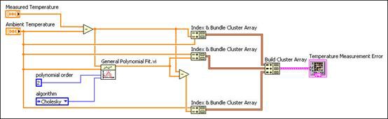
You can use the General Polynomial Fit VI to create the following block diagram to find the compensated measurement error.
Figure 10. Block Diagram of an Error Function VI Using the General Polynomial Fit VI
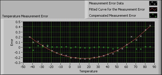
The following front panel displays the results of the experiment using the VI in Figure 10.
Figure 11. Using the General Polynomial Fit VI to Fit the Error Curve
The previous figure shows the original measurement error data set, the fitted curve to the data set, and the compensated measurement error. After first defining the fitted curve to the data set, the VI uses the fitted curve of the measurement error data to compensate the original measurement error.
You can see from the graph of the compensated error that using curve fitting improves the results of the measurement instrument by decreasing the measurement error to about one tenth of the original error value.
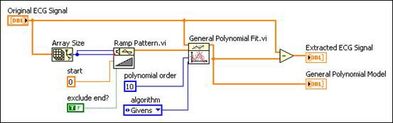
During signal acquisition, a signal sometimes mixes with low frequency noise, which results in baseline wandering. Baseline wandering influences signal quality, therefore affecting subsequent processes. To remove baseline wandering, you can use curve fitting to obtain and extract the signal trend from the original signal.
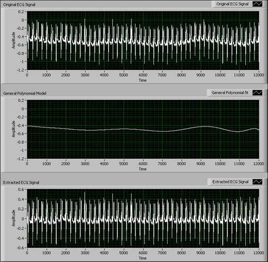
As shown in the following figures, you can find baseline wandering in an ECG signal that measures human respiration. You can obtain the signal trend using the General Polynomial Fit VI and then detrend the signal by finding and removing the baseline wandering from the original signal. The remaining signal is the subtracted signal.
Figure 12. Using the General Polynomial Fit VI to Remove Baseline Wandering
You can see from the previous graphs that using the General Polynomial Fit VI suppresses baseline wandering. In this example, using the curve fitting method to remove baseline wandering is faster and simpler than using other methods such as wavelet analysis.
In digital image processing, you often need to determine the shape of an object and then detect and extract the edge of the shape. This process is called edge extraction. Inferior conditions, such as poor lighting and overexposure, can result in an edge that is incomplete or blurry. If the edge of an object is a regular curve, then the curve fitting method is useful for processing the initial edge.
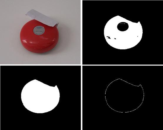
To extract the edge of an object, you first can use the watershed algorithm. This algorithm separates the object image from the background image. Then you can use the morphologic algorithm to fill in missing pixels and filter the noise pixels. After obtaining the shape of the object, use the Laplacian, or the Laplace operator, to obtain the initial edge. The following figure shows the edge extraction process on an image of an elliptical object with a physical obstruction on part of the object.
Figure 13. Edge Extraction Process
As you can see from the previous figure, the extracted edge is not smooth or complete due to lighting conditions and an obstruction by another object. Because the edge shape is elliptical, you can improve the quality of edge by using the coordinates of the initial edge to fit an ellipse function. Using an iterative process, you can update the weight of the edge pixel in order to minimize the influence of inaccurate pixels in the initial edge. The following figure shows the front panel of a VI that extracts the initial edge of the shape of an object and uses the Nonlinear Curve Fit VI to fit the initial edge to the actual shape of the object.
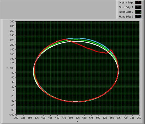
Figure 14. Using the Nonlinear Curve Fit VI to Fit an Elliptical Edge
The graph in the previous figure shows the iteration results for calculating the fitted edge. After several iterations, the VI extracts an edge that is close to the actual shape of the object.
The standard of measurement for detecting ground objects in remote sensing images is usually pixel units. Due to spatial resolution limitations, one pixel often covers hundreds of square meters. The pixel is a mixed pixel if it contains ground objects of varying compositions. Mixed pixels are complex and difficult to process. One method of processing mixed pixels is to obtain the exact percentages of the objects of interest, such as water or plants.
The following image shows a Landsat false color image taken by Landsat 7 ETM+ on July 14, 2000. This image displays an area of Shanghai for experimental data purposes.
Figure 15. False Color Image
In the previous image, you can observe the five bands of the Landsat multispectral image, with band 3 displayed as blue, band 4 as green, and band 5 as red. The image area includes three types of typical ground objects: water, plant, and soil. Soil objects include artificial architecture such as buildings and bridges.
You can use the General Linear Fit VI to create a mixed pixel decomposition VI. The following figure shows the decomposition results using the General Linear Fit VI.


(a) Plant (b) Soil and Artificial Architecture (c) Water
Figure 16. Using the General Linear Fit VI to Decompose a Mixed Pixel Image
In the previous images, black-colored areas indicate 0% of a certain object of interest, and white-colored areas indicate 100% of a certain object of interest. For example, in the image representing plant objects, white-colored areas indicate the presence of plant objects. In the image representing water objects, the white-colored, wave-shaped region indicates the presence of a river. You can compare the water representation in the previous figure with Figure 15.
From the results, you can see that the General Linear Fit VI successfully decomposes the Landsat multispectral image into three ground objects.
The model you want to fit sometimes contains a function that LabVIEW does not include. For example, the following equation describes an exponentially modified Gaussian function.
where
y0 is the offset from the y-axis
A is the amplitude of the data set
xc is the center of the data set
w is the width of the function
t0 is the modification factor
The curve fitting VIs in LabVIEW cannot fit this function directly, because LabVIEW cannot calculate generalized integrals directly. However, the integral in the previous equation is a normal probability integral, which an error function can represent according to the following equation.
represents the error function in LabVIEW.
You can rewrite the original exponentially modified Gaussian function as the following equation.
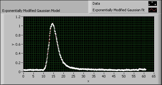
LabVIEW can fit this equation using the Nonlinear Curve Fit VI. The following figure shows an exponentially modified Gaussian model for chromatography data.
Figure 17. Exponentially Modified Gaussian Model
This model uses the Nonlinear Curve Fit VI and the Error Function VI to calculate the curve fit for a data set that is best fit with the exponentially modified Gaussian function.
By using the appropriate VIs, you can create a new VI to fit a curve to a data set whose function is not available in LabVIEW.
Curve fitting not only evaluates the relationship among variables in a data set, but also processes data sets containing noise, irregularities, errors due to inaccurate testing and measurement devices, and so on. LabVIEW provides basic and advanced curve fitting VIs that use different fitting methods, such as the LS, LAR, and Bisquare methods, to find the fitting curve. The fitting model and method you use depends on the data set you want to fit. LabVIEW also provides preprocessing and evaluation VIs to remove outliers from a data set, evaluate the accuracy of the fitting result, and measure the confidence interval and prediction interval of the fitted data.
Refer to the LabVIEW Help for more information about curve fitting and LabVIEW curve fitting VIs.